Mass-Spring-Damper
Introduction
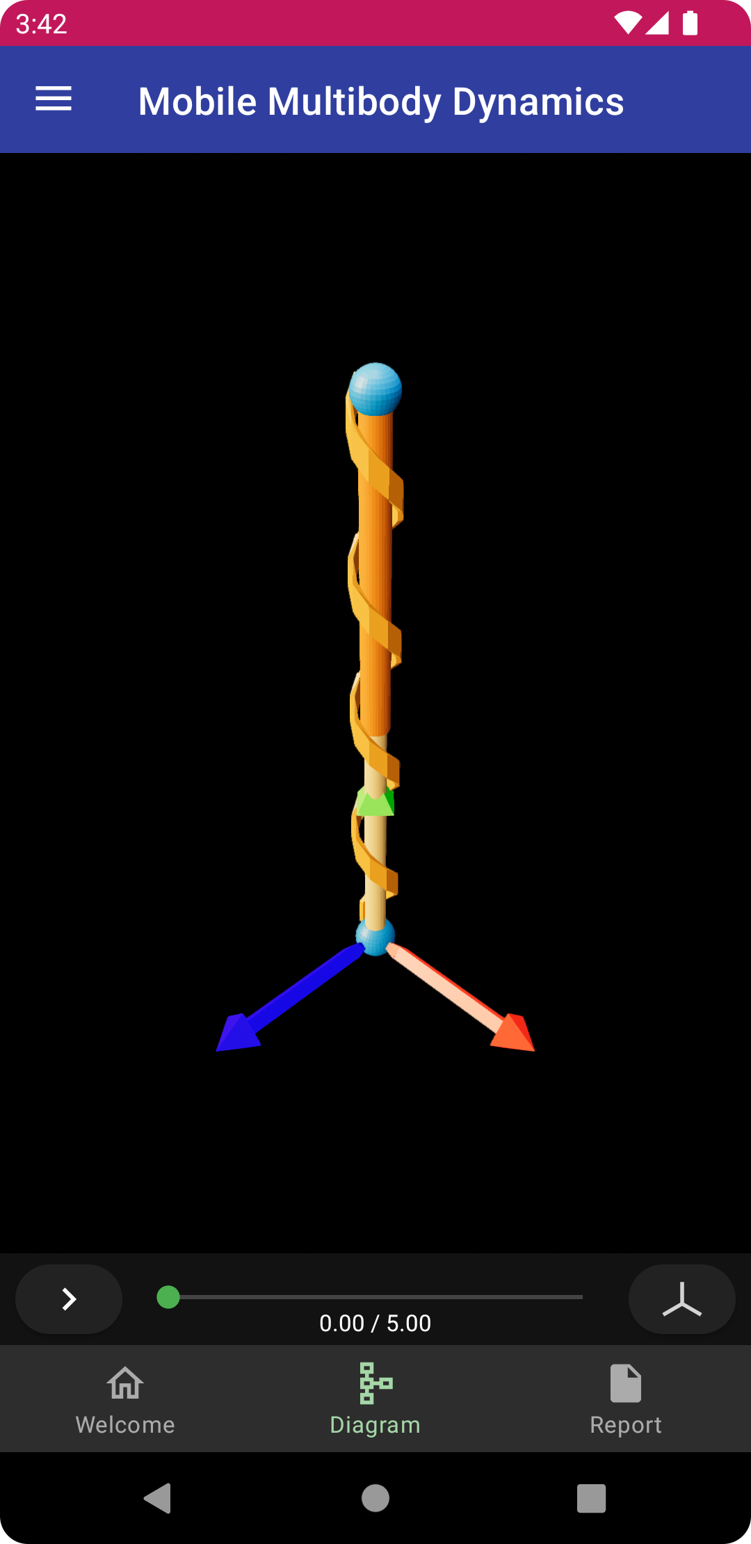
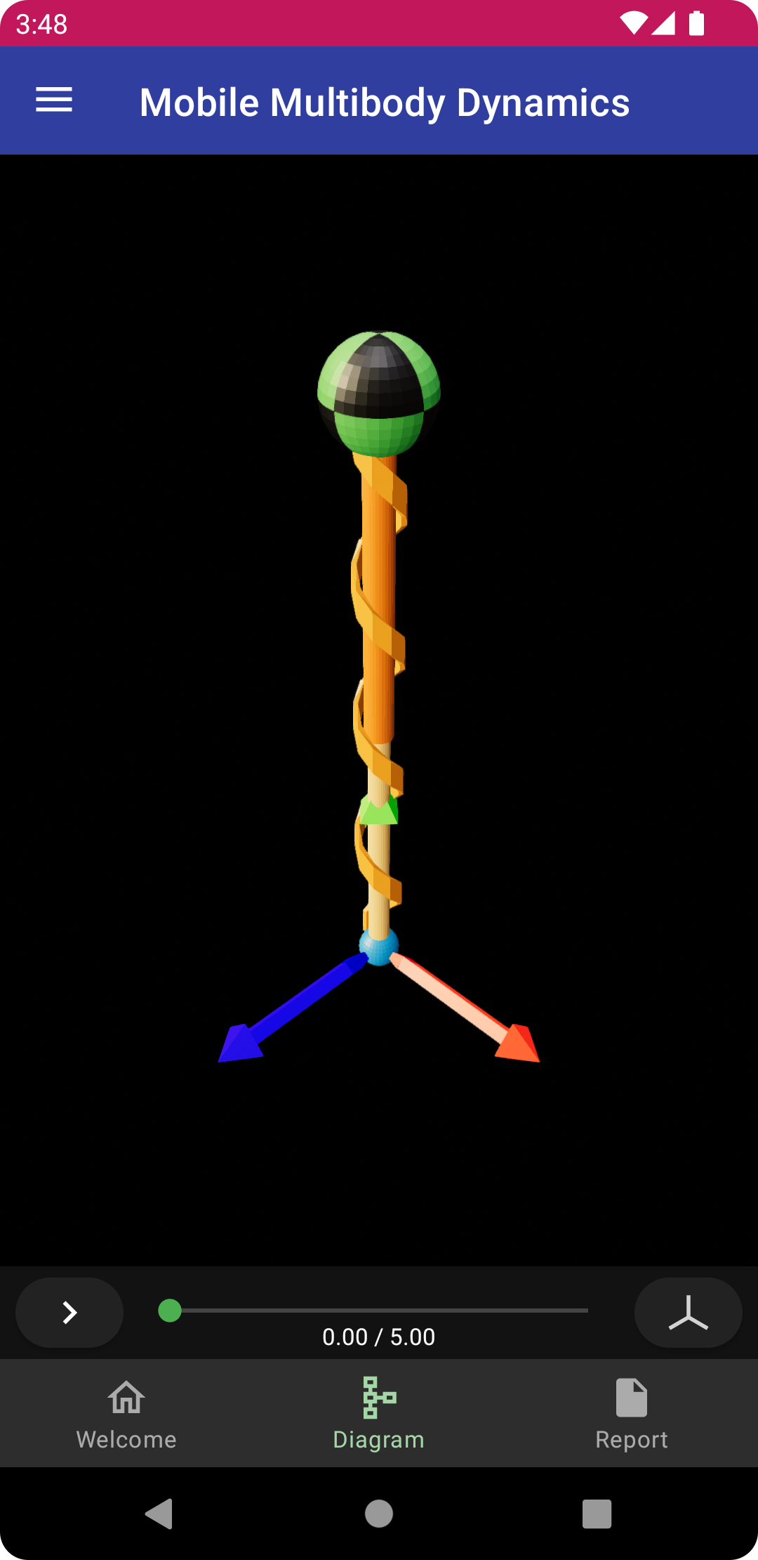
This is a tutorial for creating a mass-spring-damper system in a uniform gravitational field, which is the fundamental problem used in study of linear vibration. The animation below is generated in MOMDYN at the completion of the tutorial. You can also watch a video demonstration of this tutorial on Youtube.
The model is generated using two variations on the kinematics interface, “Classic,” and “Joints.” The former is akin to a pencil-and-paper approach, each symbolic parameter is individually named by the user, and each frame, vector, and point is created using these parameters. The latter is closer to the approach used in modern multibody dynamics software, where lower-level modeling attributes are consolidated into a prismatic joint object, reducing the total number of steps.
New Model
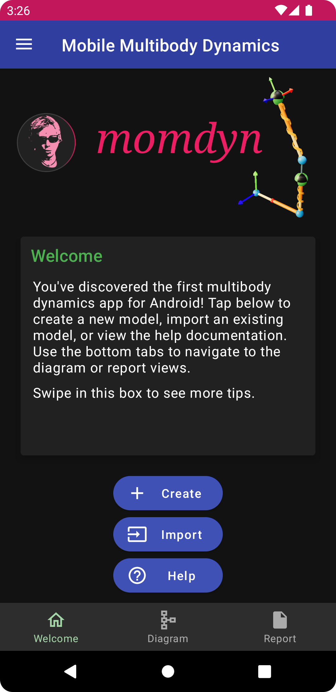
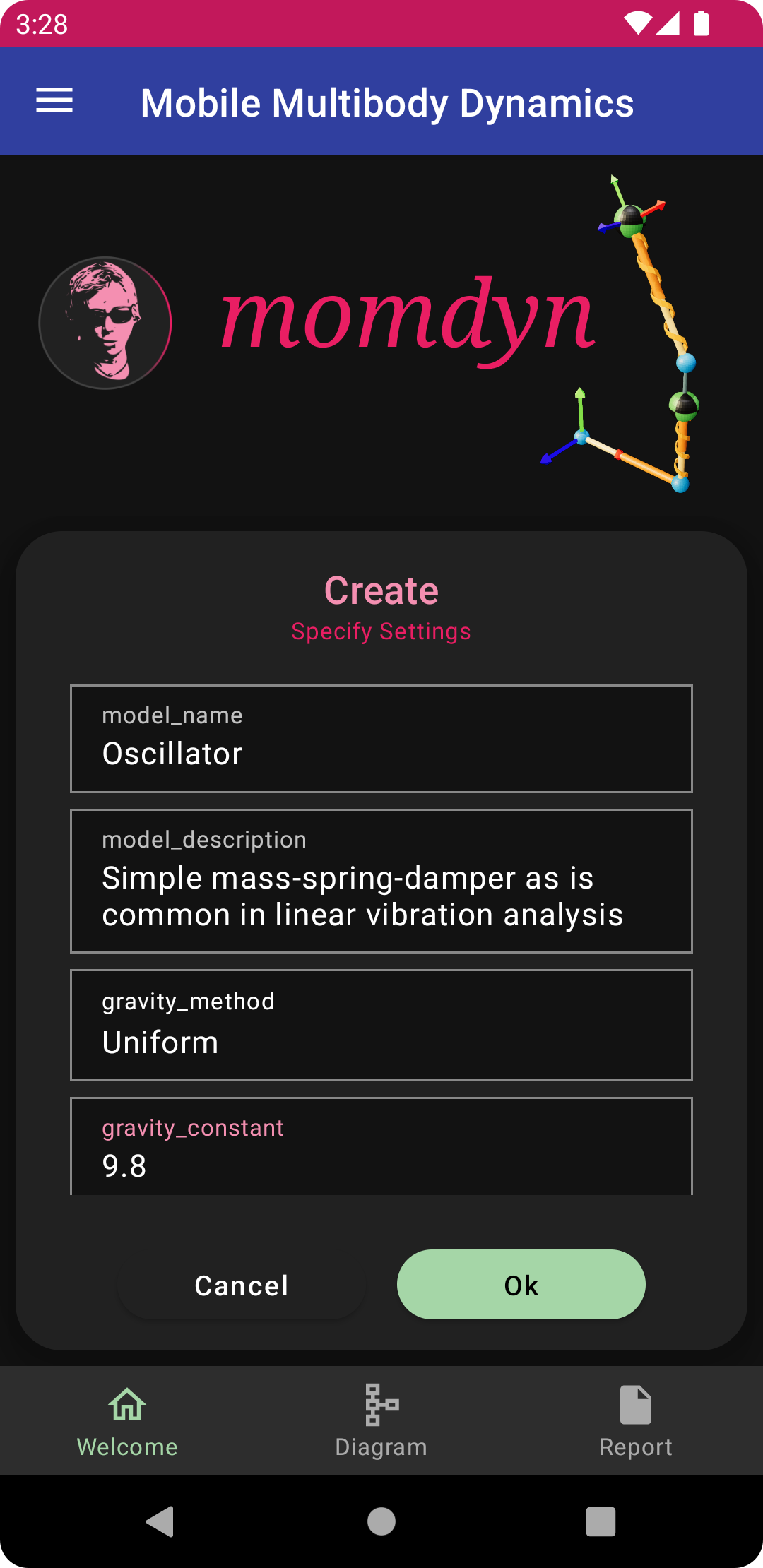
To begin, from the welcome screen tap the “Create” button, which will bring up a dialog with the title “Create - Specify Settings.” Many of the settings in this dialog can remain with their defaults. The modified specifications give a model name and description, and creates gravitational force, time, and tolerance. Enter the following:
model_name: Oscillator
model_description: Simple mass-spring-damper as is common in linear vibration analysis
gravity_method: Uniform
gravity_constant: 9.8
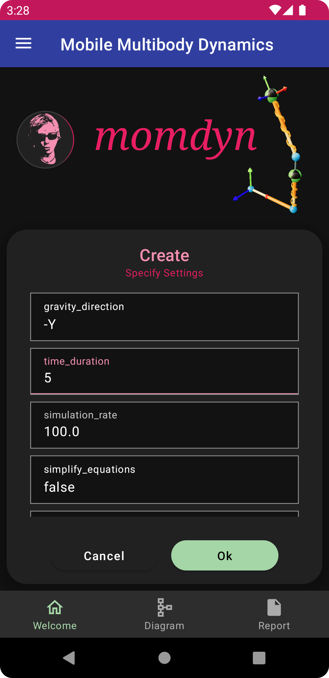
gravity_direction: -Y
time_duration: 5
tol: 0.00001
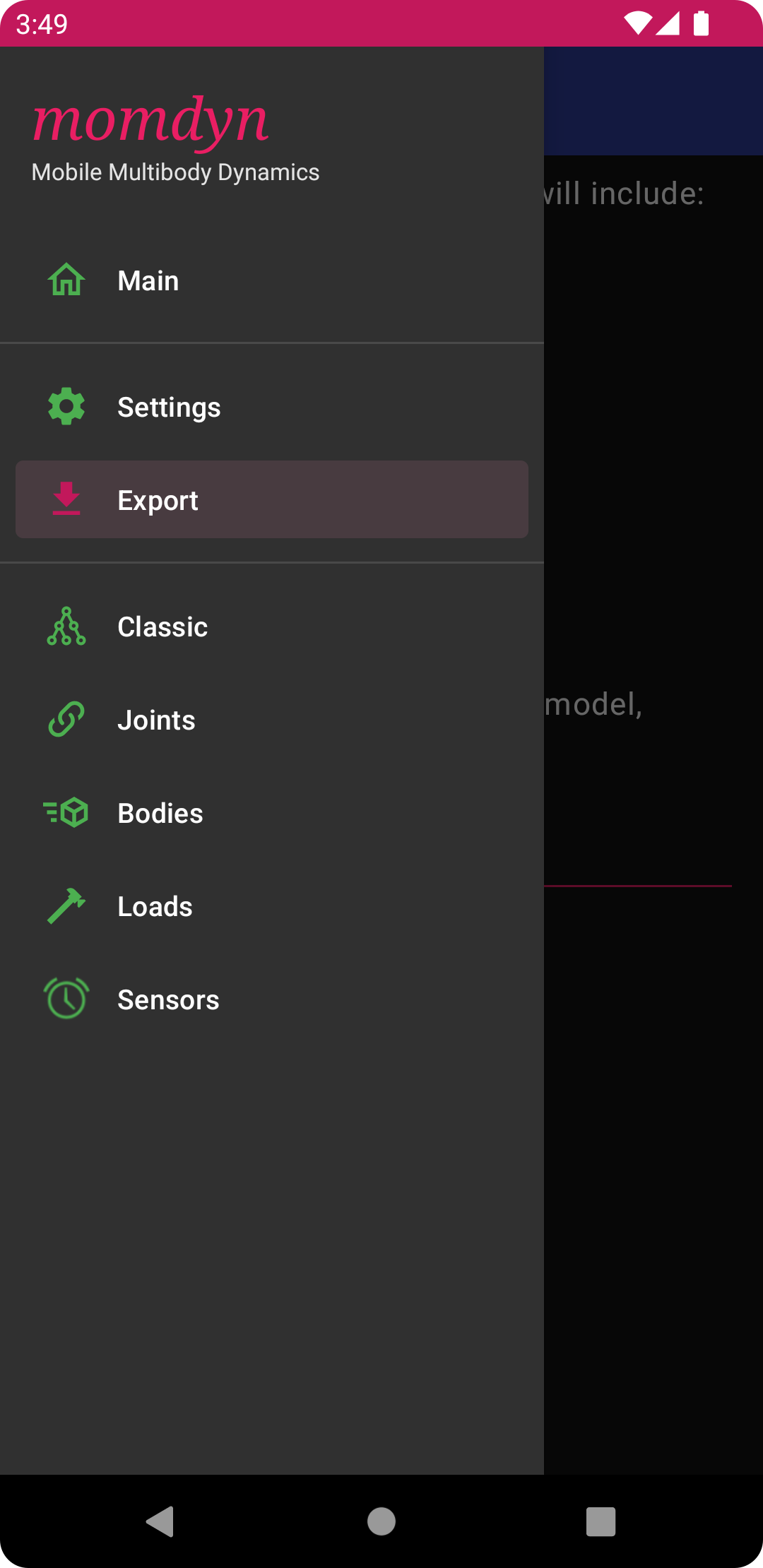
Tap the “Ok” button to create the model. Open the navigation drawer by tapping the button in the upper left, and then tap the export menu option. Tap the “Export Now” button to save the model. as we will be returning to this stage later in the tutorial.
Classic Interface
Here we will use the classic interface, which allows for more direct control over the fundamental building blocks of the kinematics. Here we will define a generalized coordinate for displacement, attach that generalized coordinate to a vector, and create a point defined relative to the origin by the vector. The spring is defined that connects the origin and created point, with stiffness, damping, and equilibrium properties.
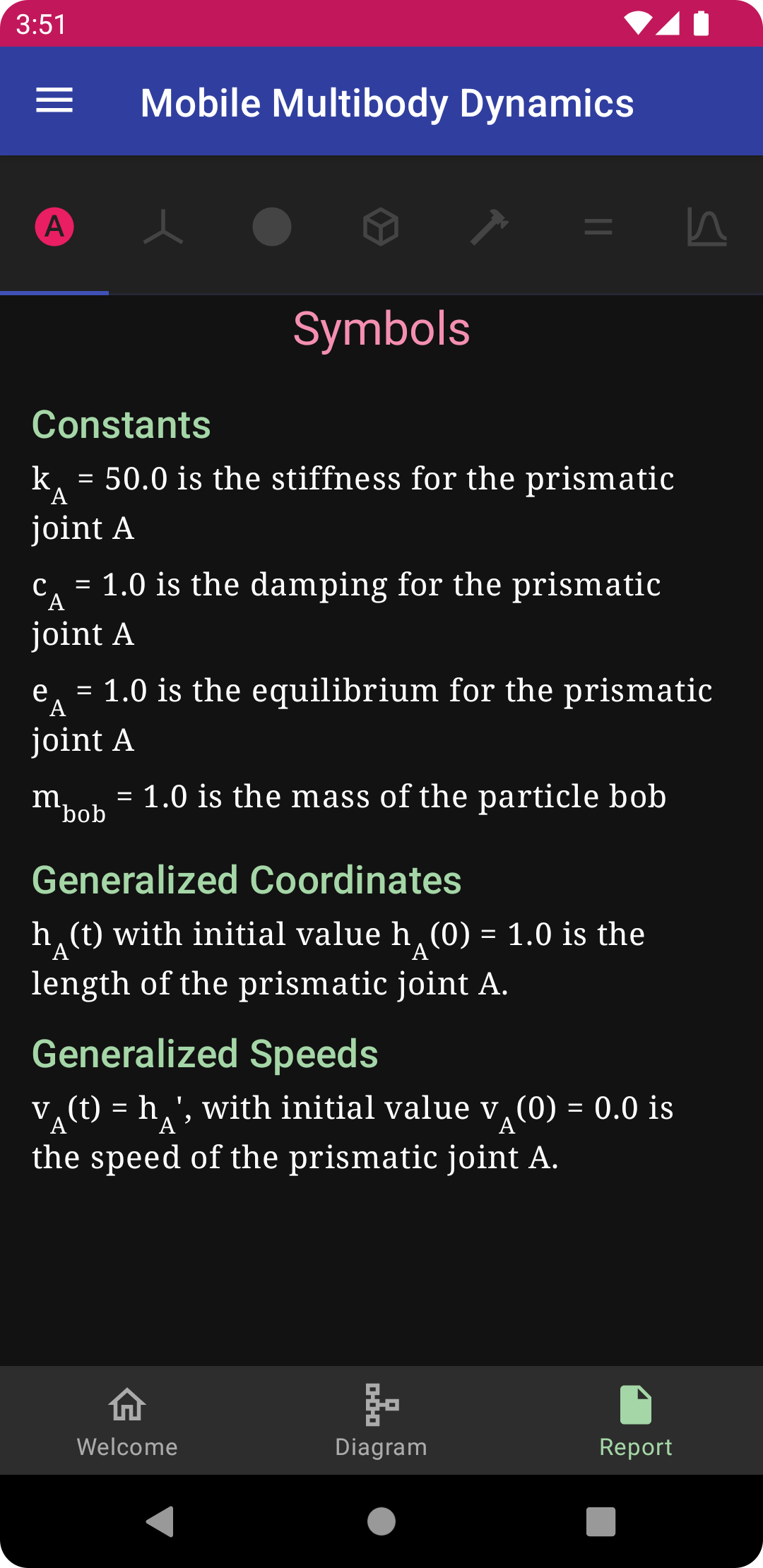
Create Symbols
For this model, a single time-varying generalized coordinate is defined representing displacement. The creation of constants for spring stiffness, damping, and equilibrium is done automatically in the translational spring object which will be created later in this tutorial.
Generalized Coordinate
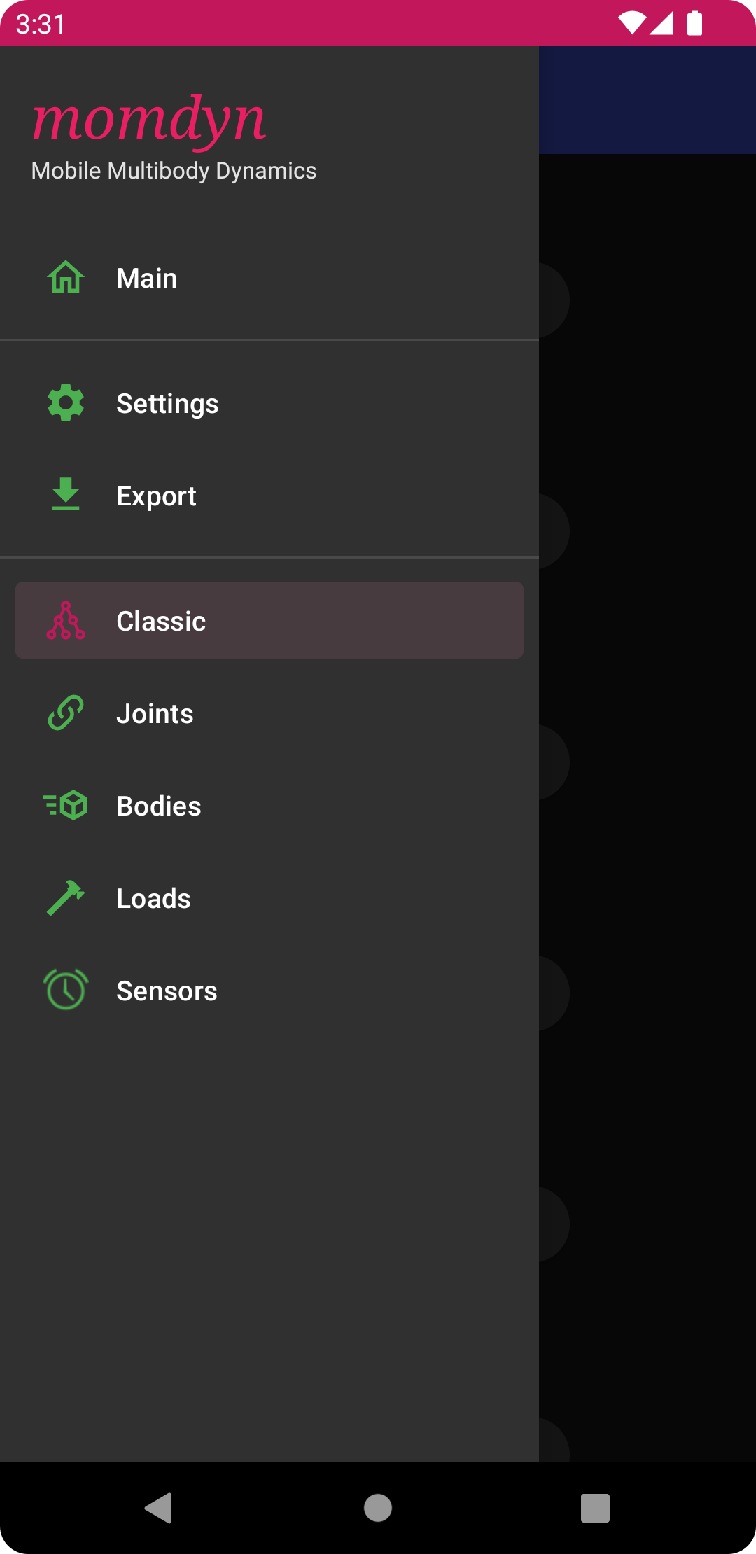
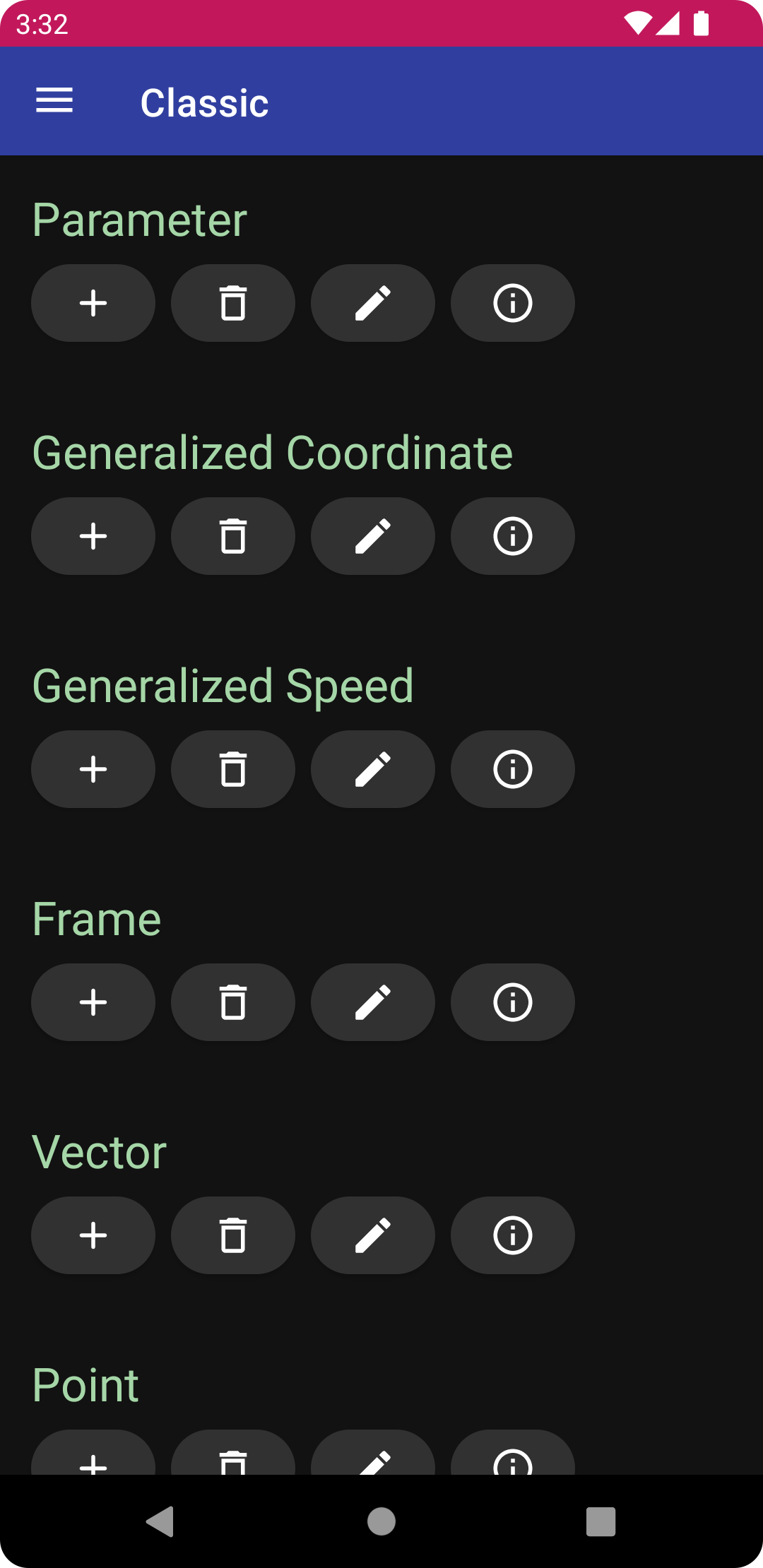
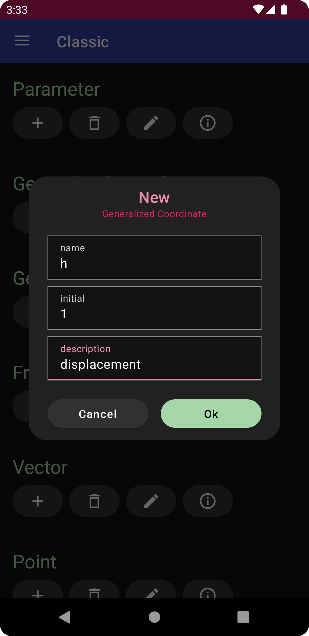
Open the navigation drawer, and then select the classic menu option. Tap the plus sign under generalized coordinate, and enter the following specifications for a translational degree of freedom.
name: h
initial: 1
description: displacement
Tap “Ok” to create the displacement coordinate.
Kinematics
The kinematics in this tutorial are established using a single vector and point that is positioned relative to the origin by the created vector.
Vector
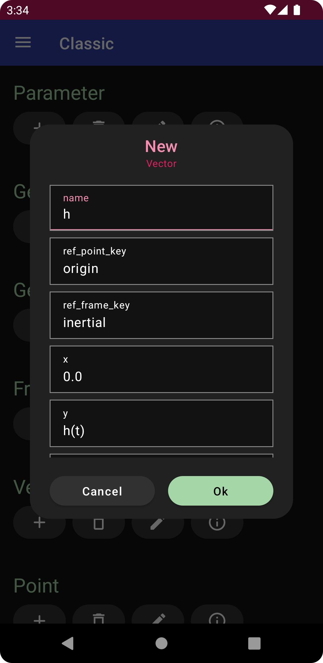
Next, with the classic panel open, tap the plus sign under vector, and enter the following
name: h
y: h(t)
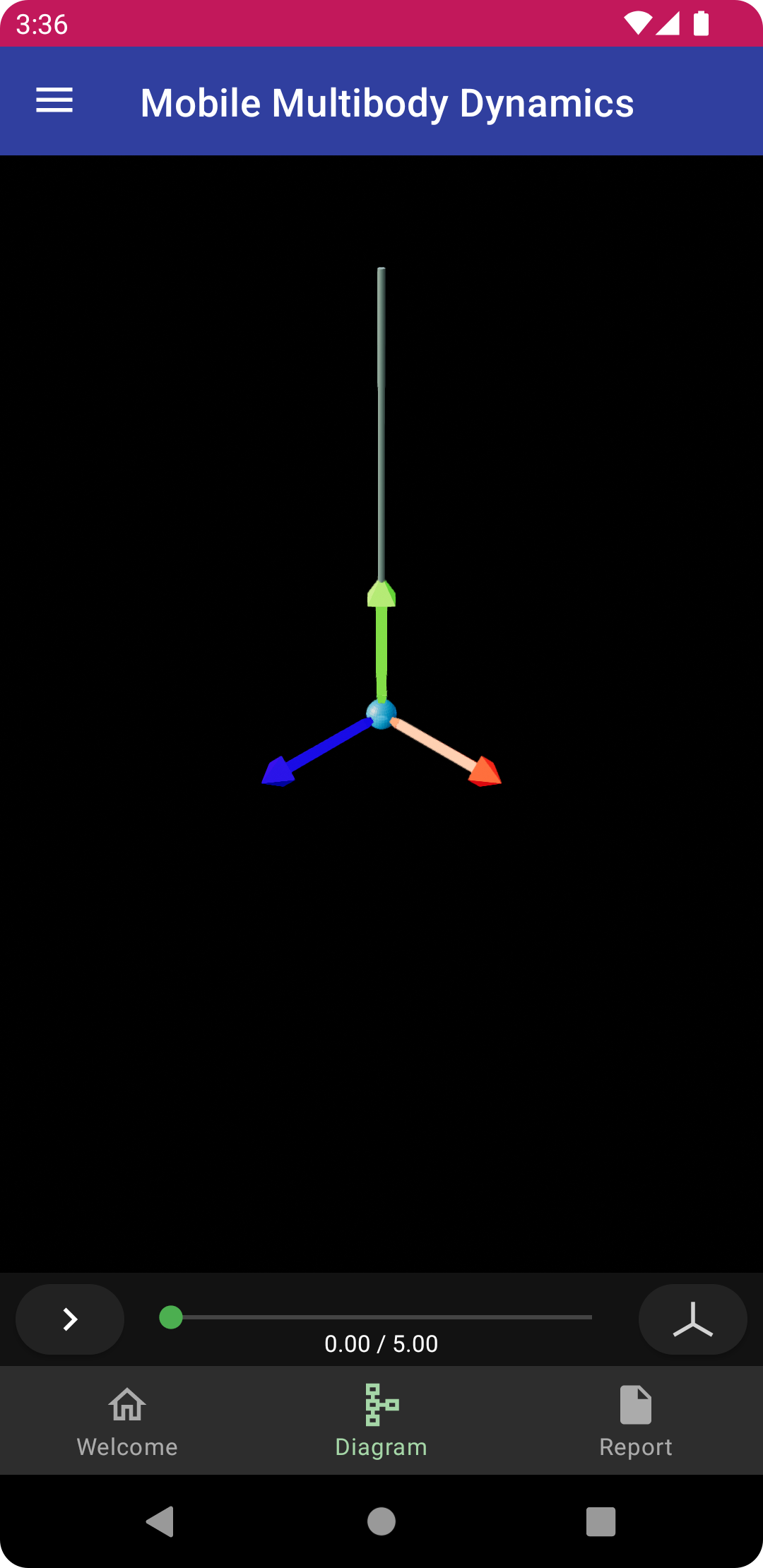
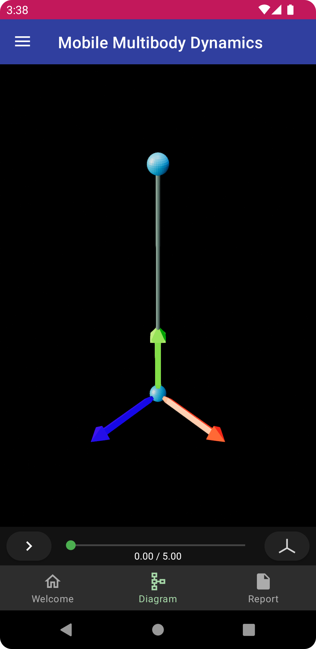
and tap the “Ok” button to create the vector named h, aligned with the j axis of the inertial frame, with length equal to the generalized coordinate h. Return to the diagram view to see the vector rendered as a gray line.
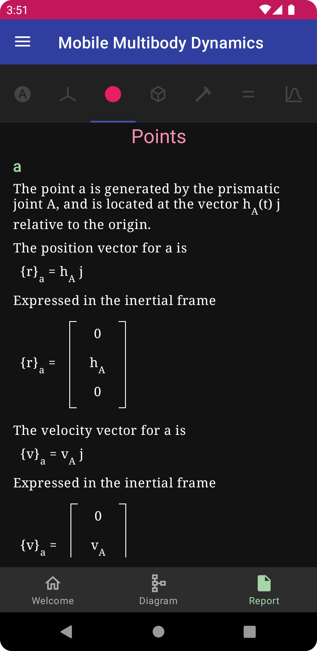
Point
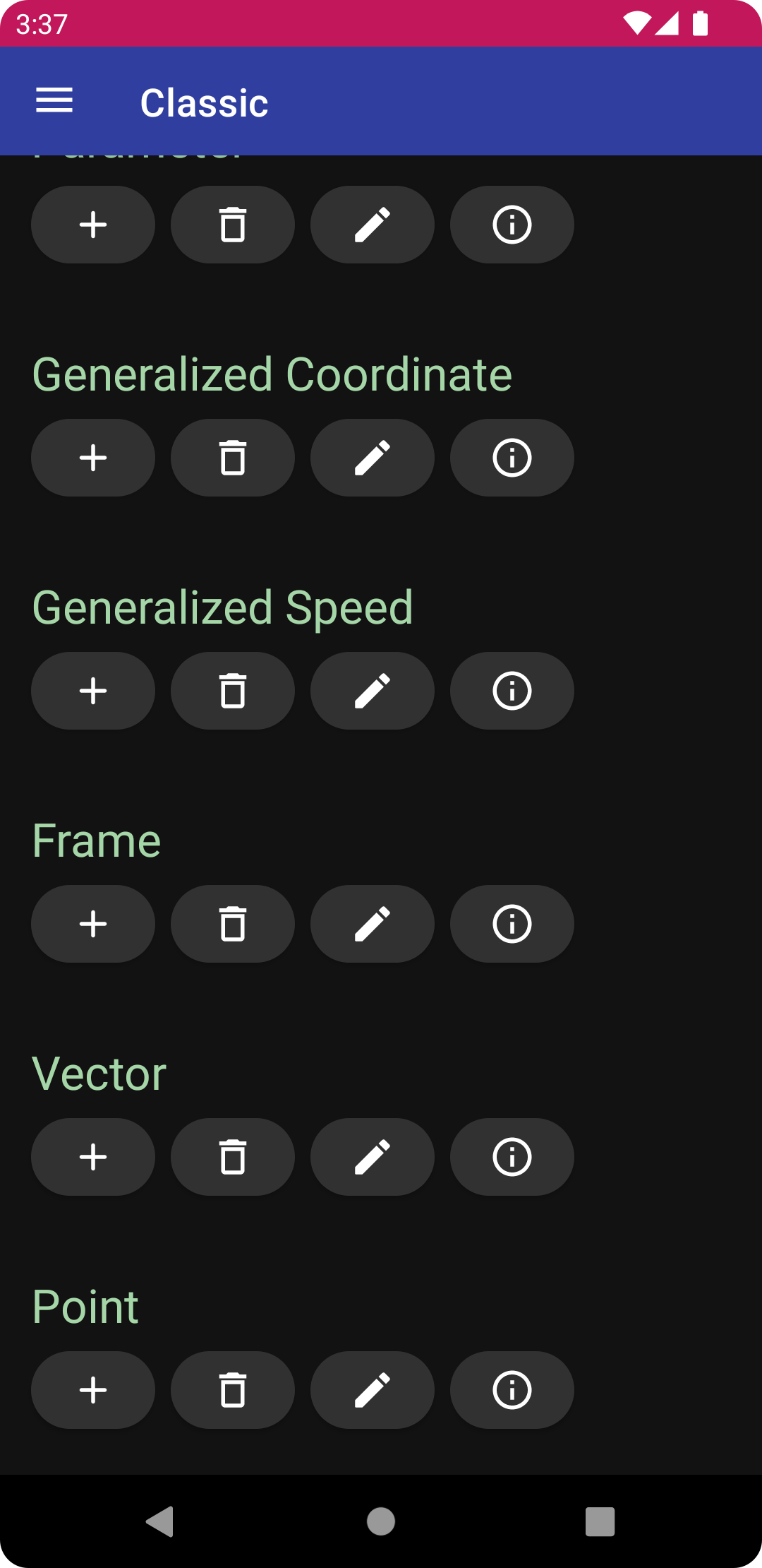
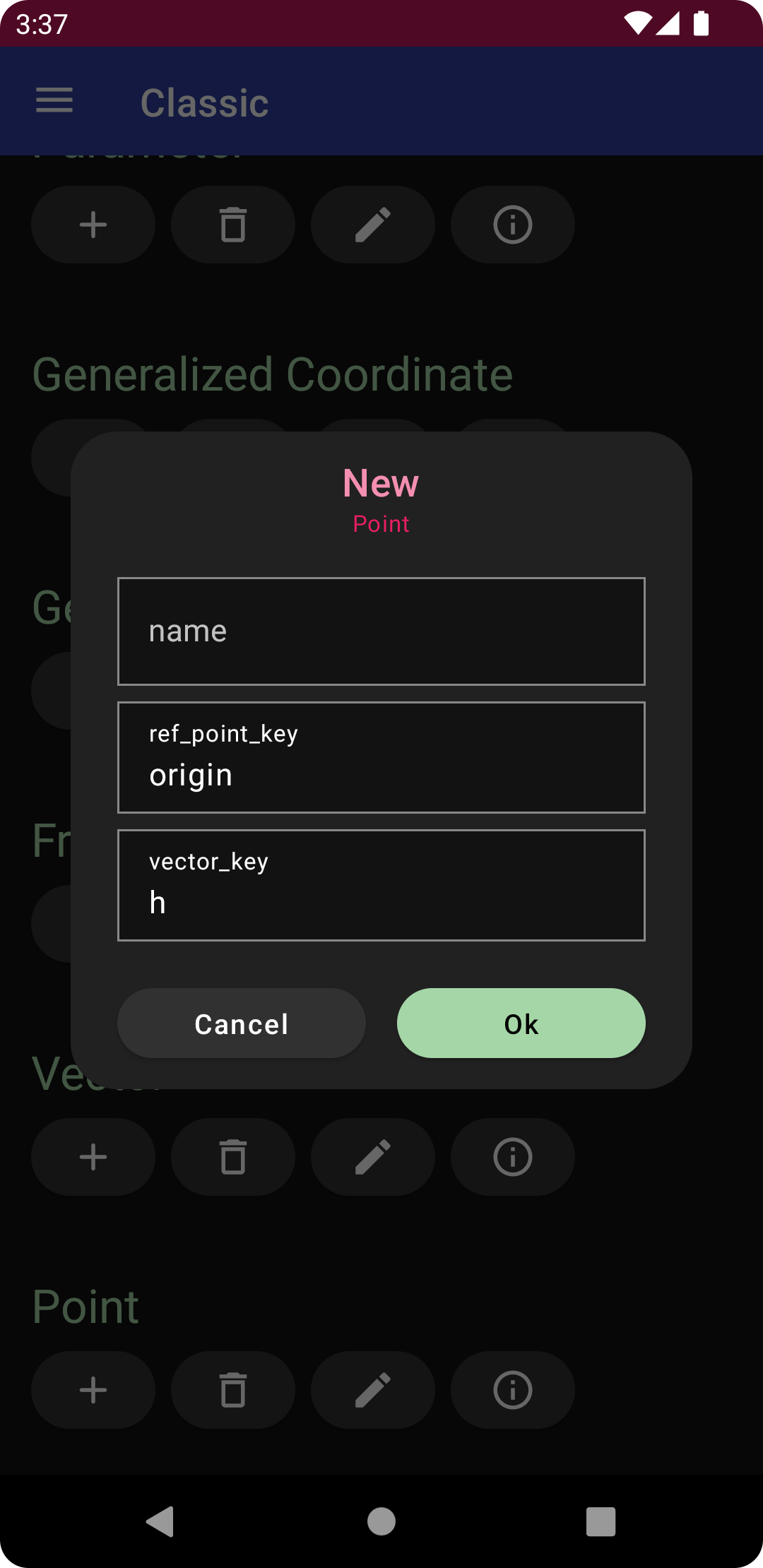
Next, tap the plus sign under point, and enter the following
vector_key: h(t)
and tap the “Ok” button to create the point a at the end of the vector h. Return to the diagram view, where you will see the diagram updated to include the new vector and point, with the latter rendered as a blue sphere.
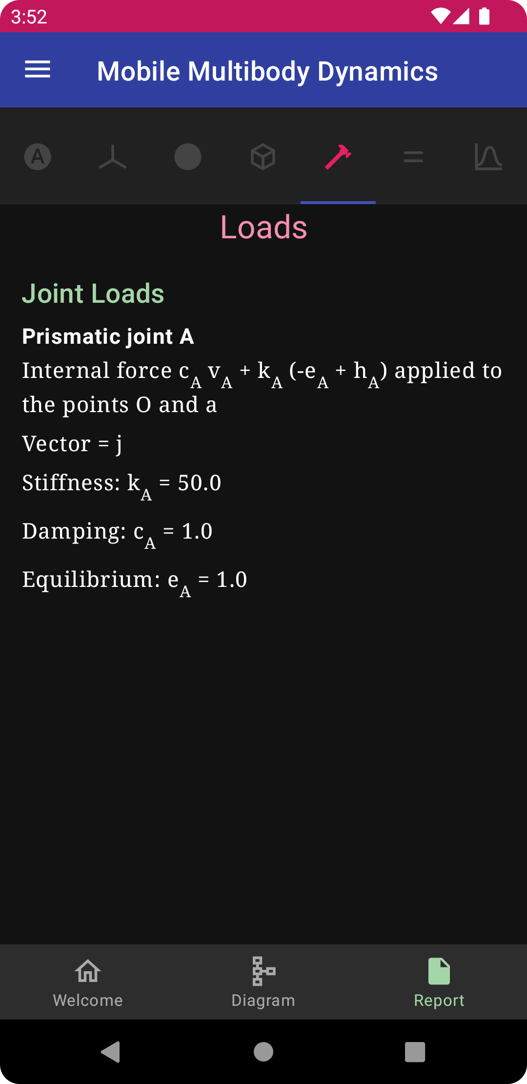
Loads
A single load is applied in this model as a spring force applied equally and in opposite directions to the origin and the created point. The spring force is proportional to stiffness times the point’s displacement relative to its equilibrium, and damping times the velocity of the point.
Translational Spring
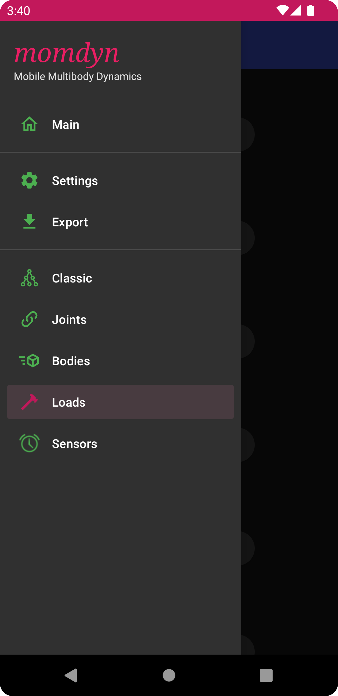
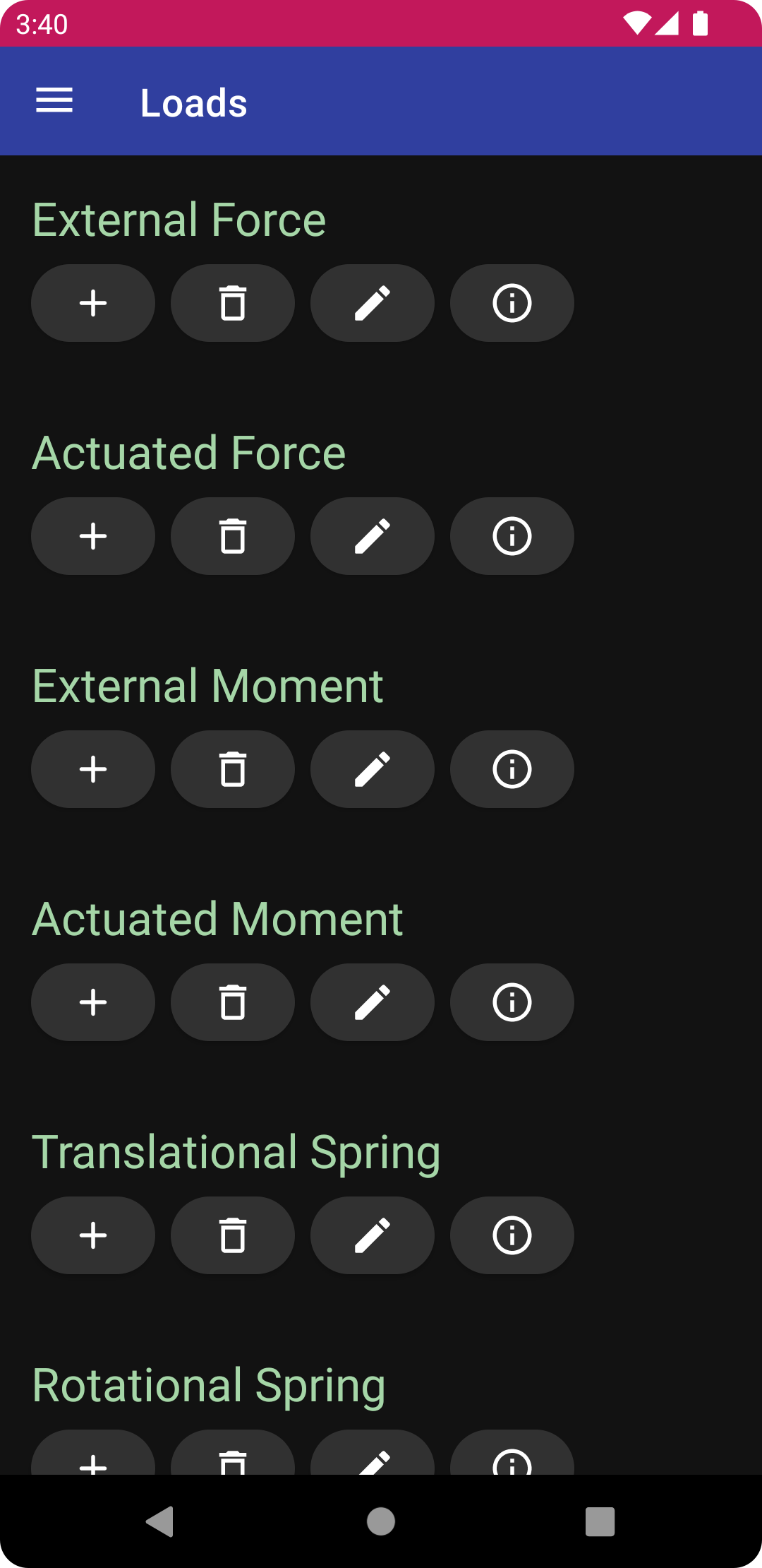
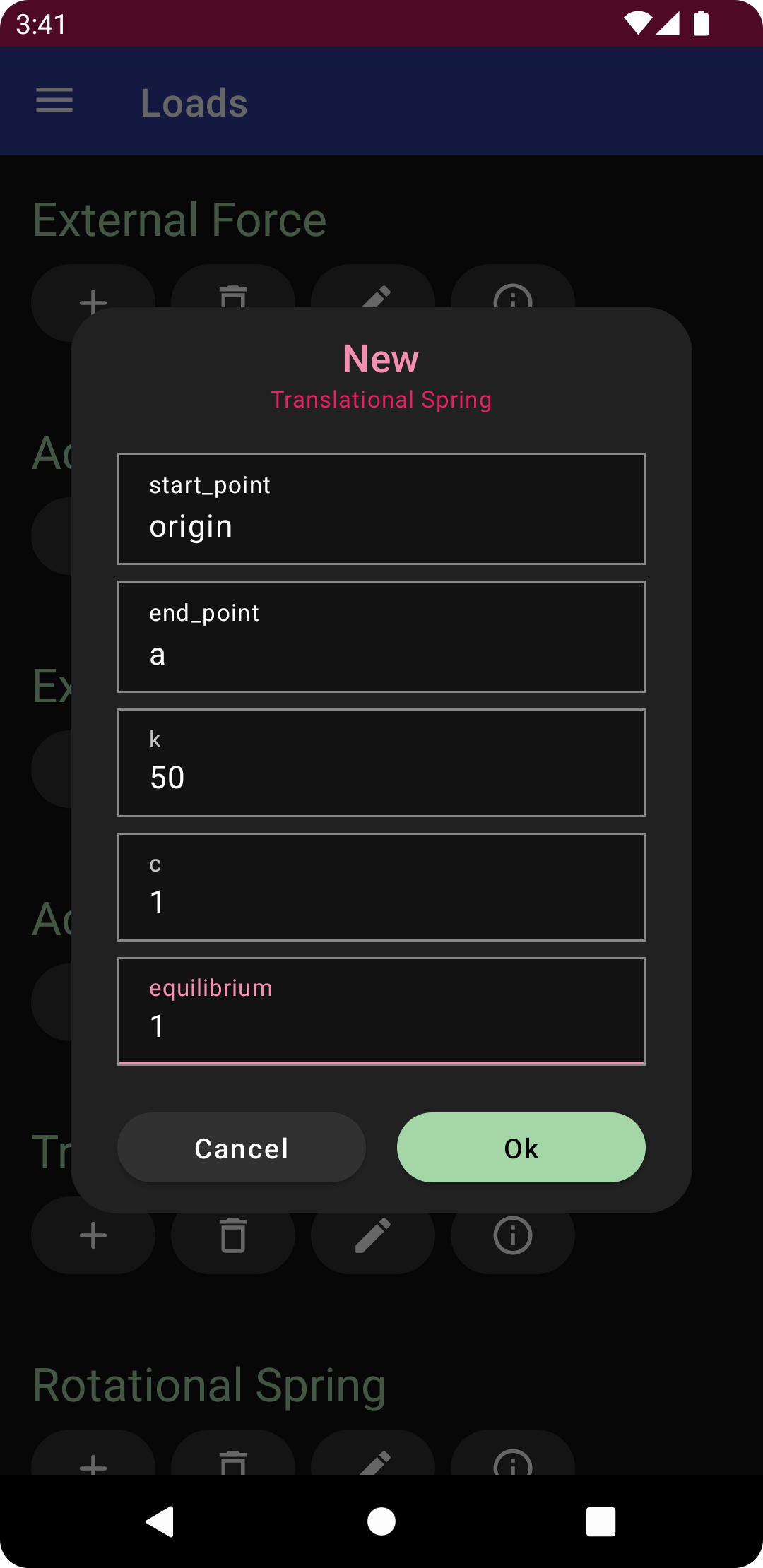
From the navigation drawer, tap the loads menu option, and then tap the plus icon under translational spring. Enter the following
end_point: a
k: 50
c: 1
equilibrium: 1
then tap the “Ok” button to create the spring. This will additionally create the parameters kO/a, cO/a, and eO/a, for stiffness, damping, and equilibrium, respectively. Return to the diagram, where you will see the spring rendered between the two points.
Joints Interface
The joints interface is more convenient for many applications, as it consolidates functionality of the building block components into common mechanical joints, and doesn’t require individually defining all of the symbols, vectors, and points in the model. In this case, the displacement coordinate, vector, point, and spring are all contained in a single prismatic joint object.
Prismatic Joint
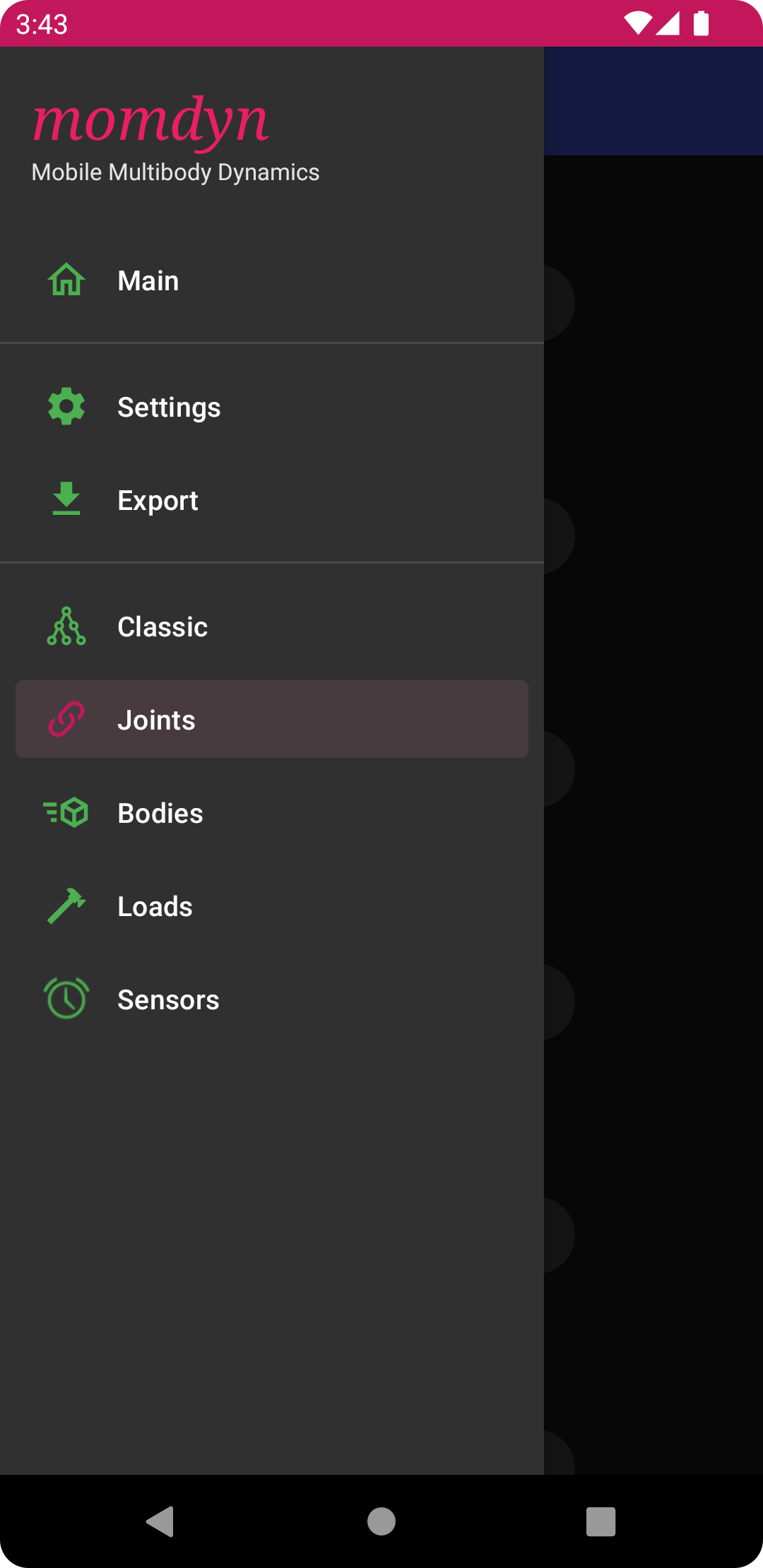
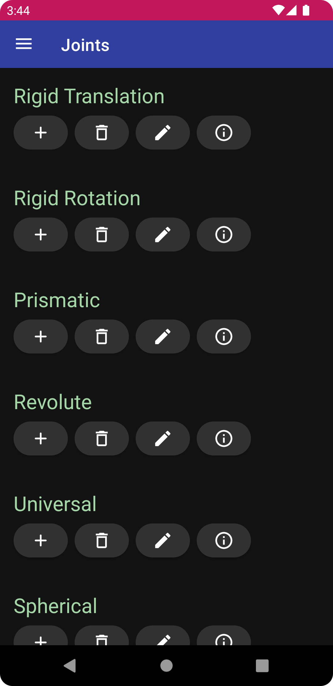
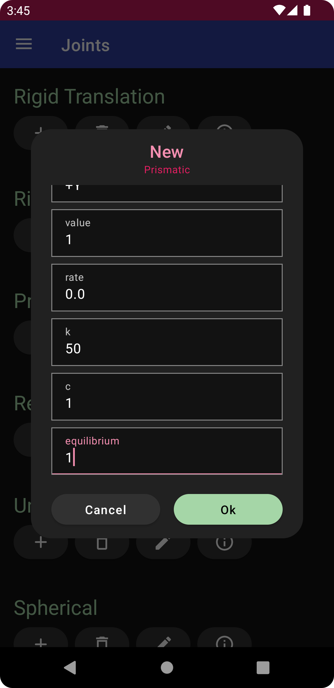
Tap on the welcome tab on the bottom of the screen, then the import button, and select the saved Oscillator file, which will return the model to its original state. Open the navigation drawer, and tap the joints menu item, then tap the plus sign under prismatic. Add the following specifications, leaving line items that are unlisted at their default value,
y: 1
value: 1
k: 50
c: 1
equilibrium: 1
and then tap the “Ok” button to create the joint. Return to the diagram to see the created point and spring in the same configuration as defined after completion of the classic procedure.
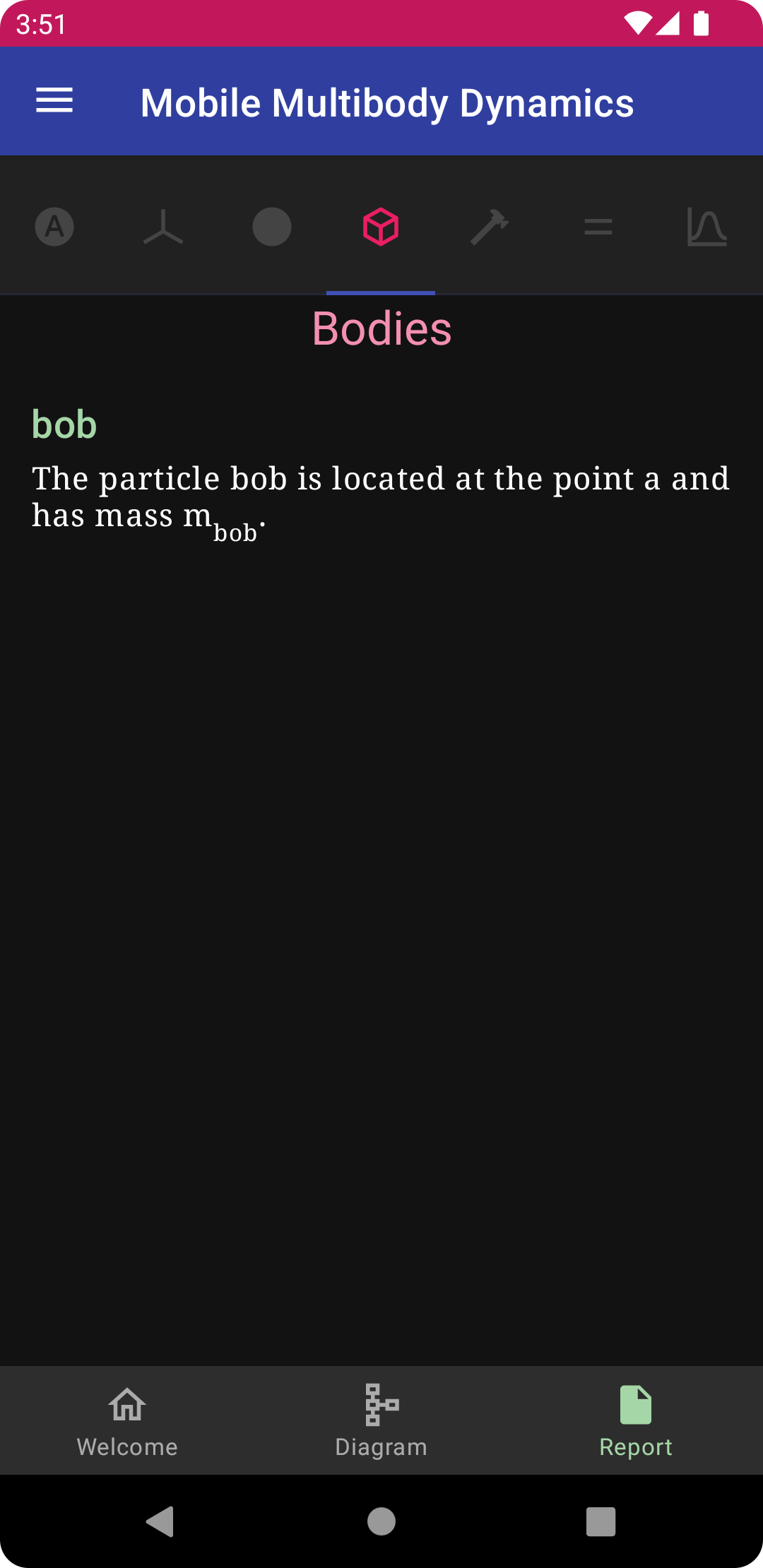
Bodies
A single particle (or point mass) is defined and attached to the created point. The inertial (or internal) force on this body will be proportional to its mass times acceleration.
Particle
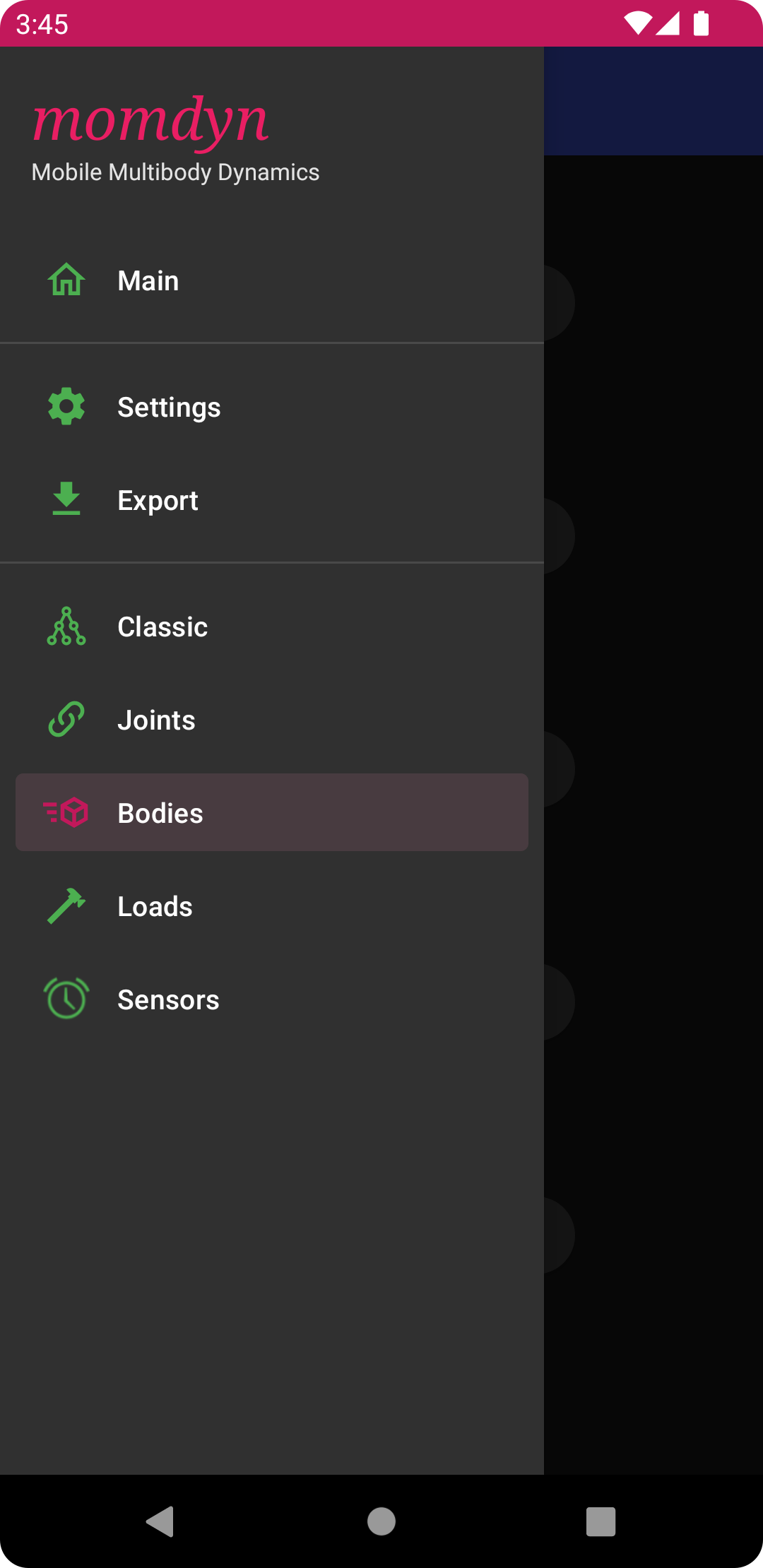
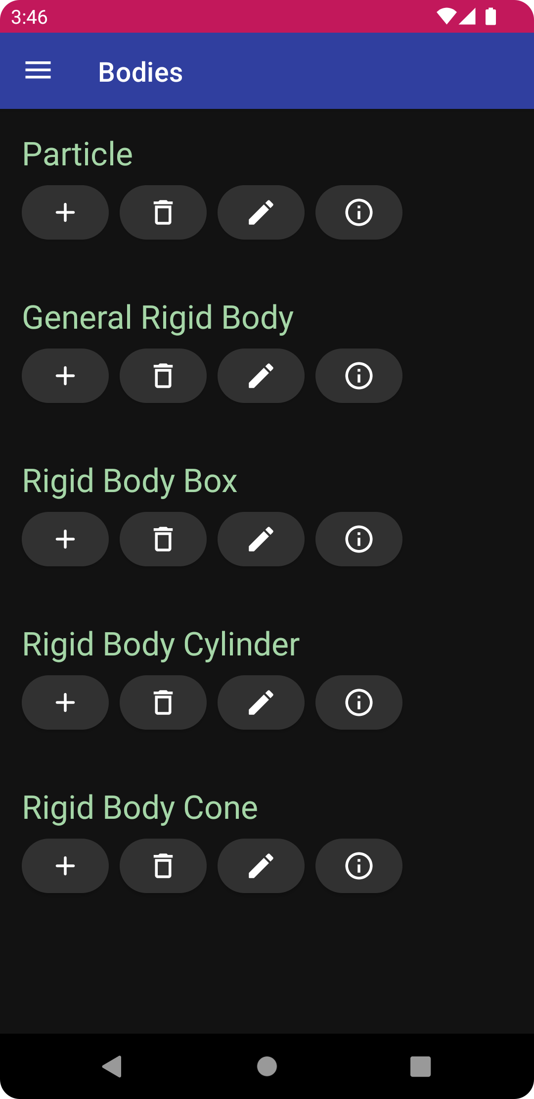
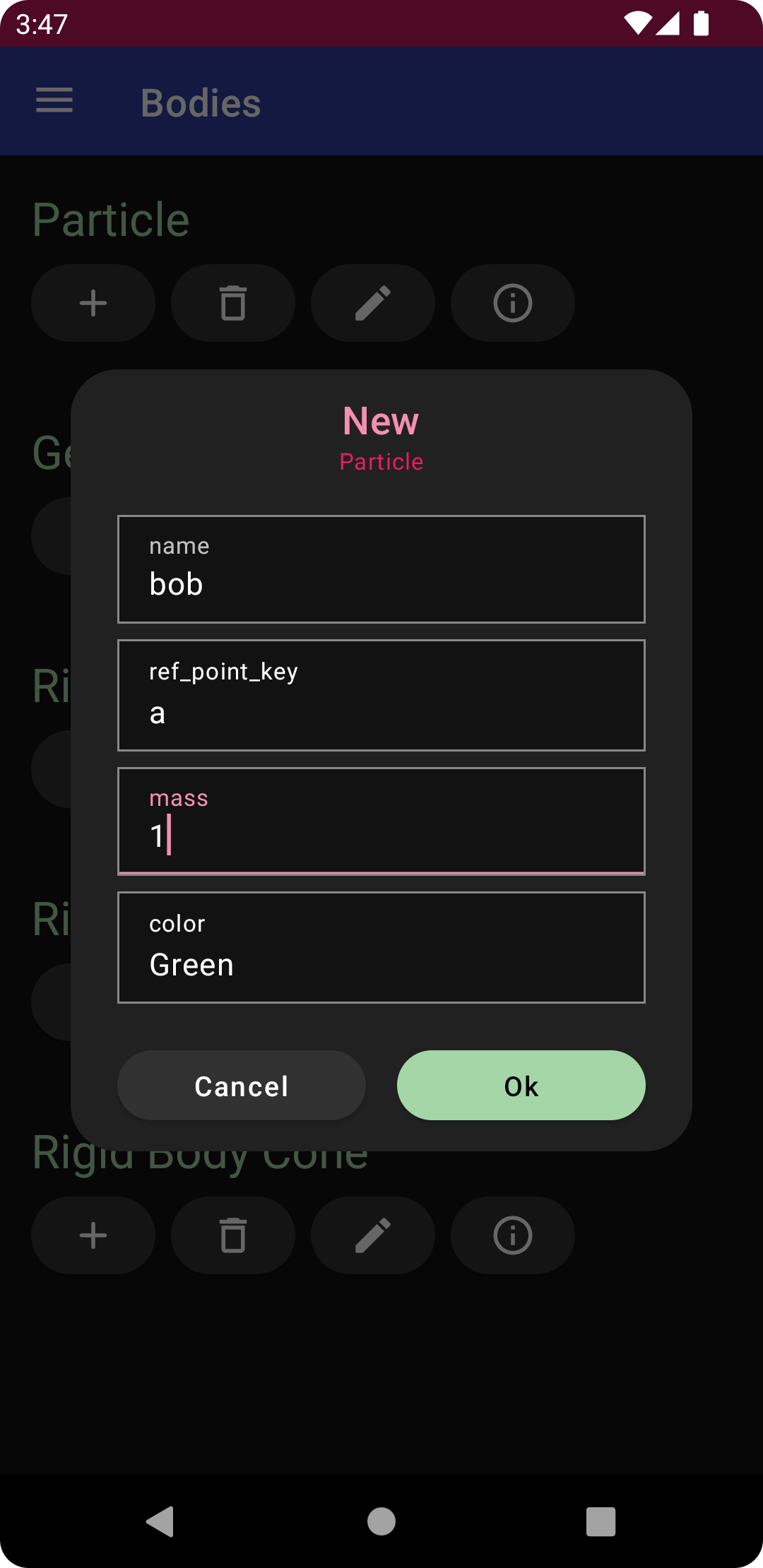
Open the navigation drawer and select the bodies menu. Tap on the plus sign under particle, and enter the following.
name: bob
ref_point_key: a
mass: 1
which will create the bob with mass of 1 attached to the point a, as shown. Additionally, the parameter mbobwill be created. Return to the diagram to see the created particle rendered as a green and black sphere.
Analysis
Here we will demonstrate the simulation and animation features, as well as the report containing documentation of the modeling parameters, system equations, and plots of the motion states. We will also show the export feature, which will save the model for future use, and create output data, plots, and Python code.
Simulation
To generate equations of motion, tap the right-arrow button in the lower left corner of the diagram. Since this is a very simple model, the derivation runs nearly instantaneously. Once complete, the icon will change to the outline of a play button. Tap again to run the simulation, once again this will be nearly instantaneous. Tap again to play the animation, which will show the mass bouncing with around a 1 second period, as seen previously at the top of this page.
Model Export
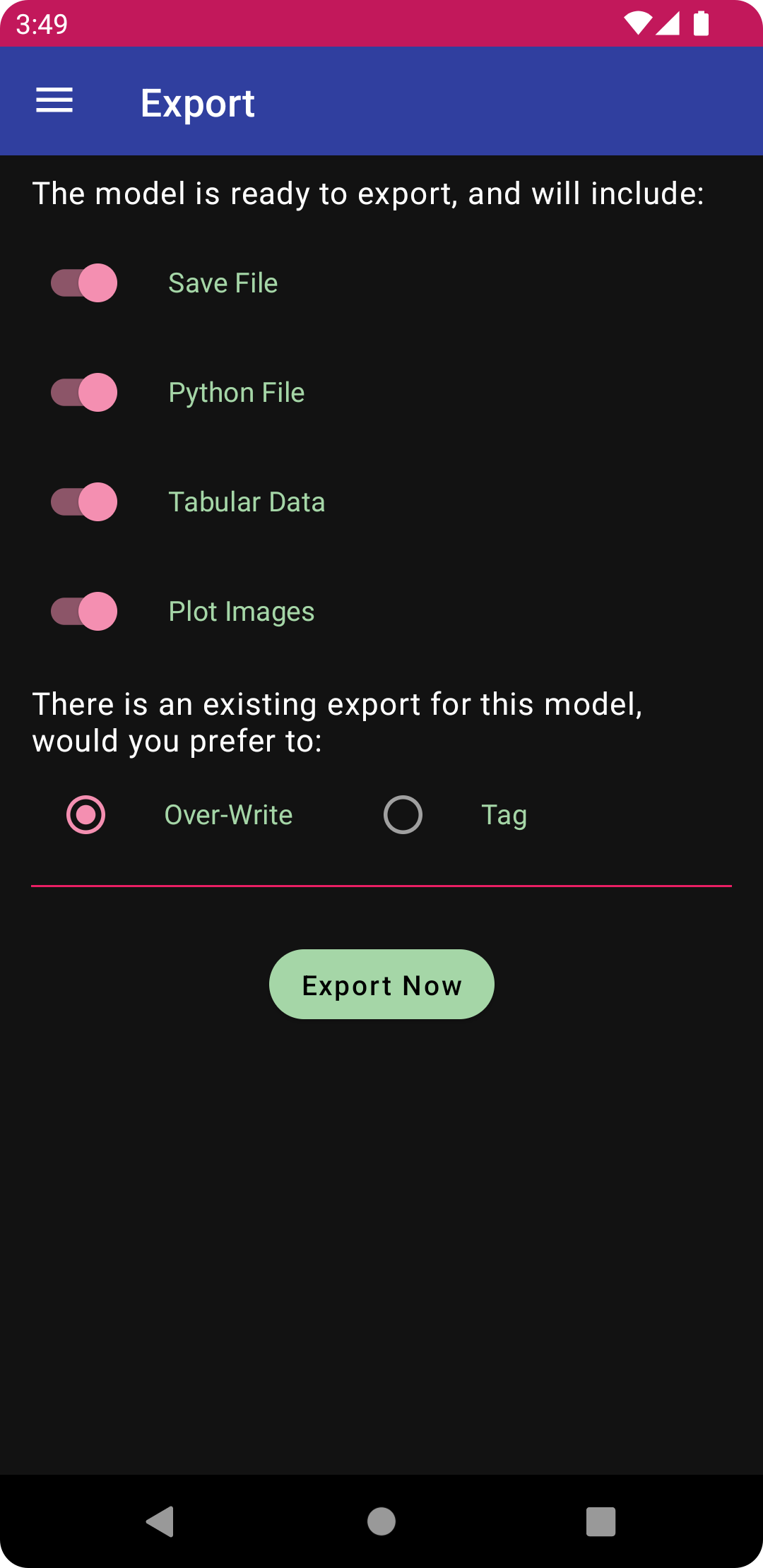
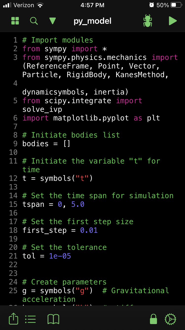
Open the navigation drawer by tapping the three horizontal lines in the upper left corner, and then tap on the export button. Keep each of the items selected, as is default, then tap the “Export Now” button to export the files. The Model file (momdyn_model.py) is the format used to import to the MOMDYN app. The Simulation file (simulation.csv) are the time-series reflecting the generalized coordinates and speeds that are animated. The Python file (py_model.py) contains code that can be executed and further manipulated on a desktop Python environment.
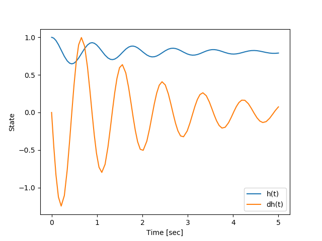
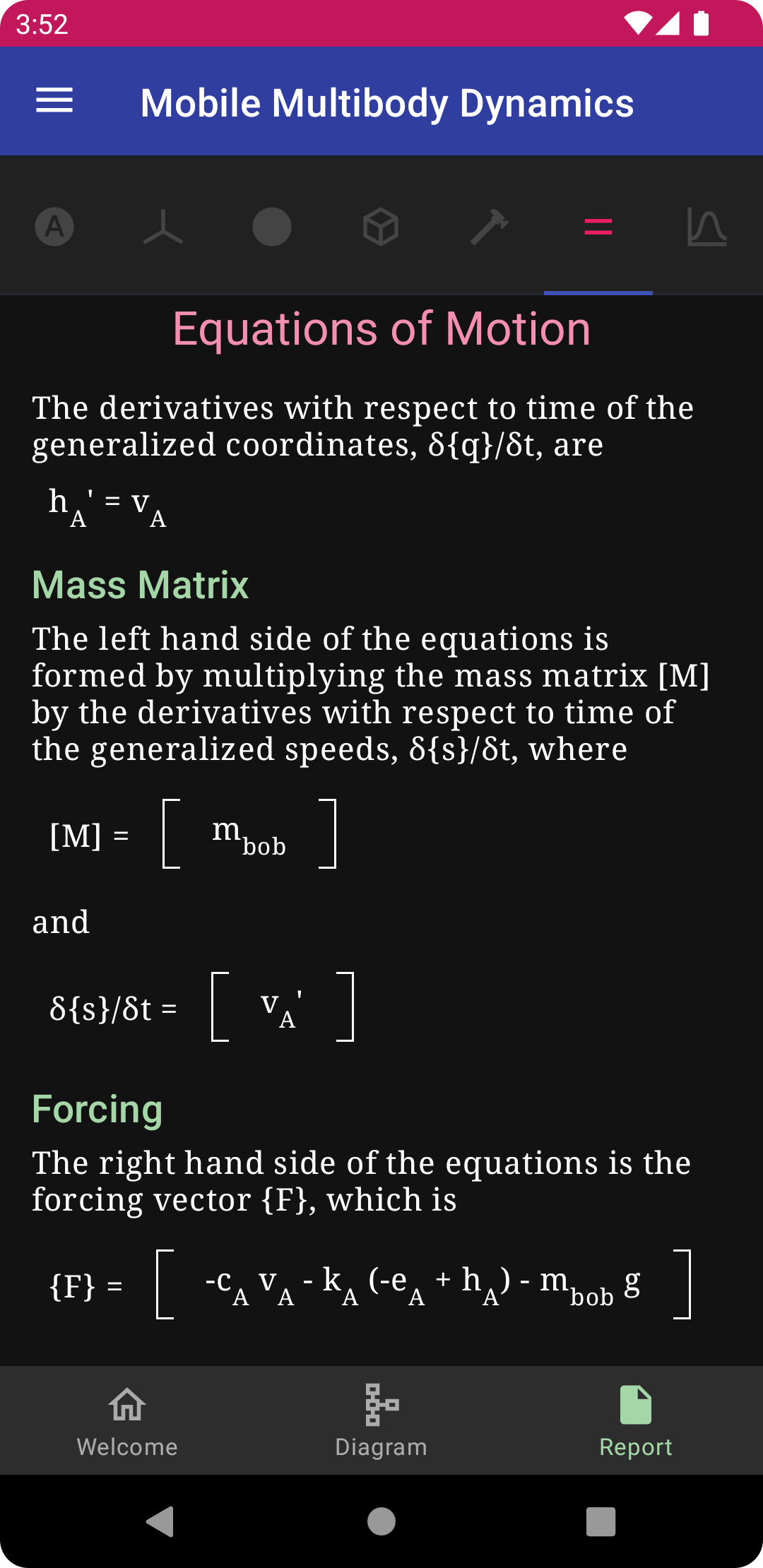
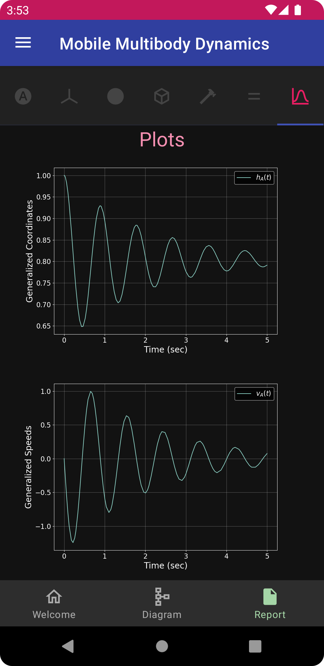
Report
Tap on the report tab in the lower right to open up the report view showing text, equations and plots. The buttons at the top specify which section of the report to view. From left to right these are symbols, frames, points, bodies, loads, equations, and plots. The images below show these sections for the Oscillator model, omitting frames as there are none (except for the inertial frame).